

Forecasting the Second Coming
How a mathematician in 1699 calculated when Jesus would return

Temporis spatium definire, in quo Historiae Christi scriptae probabilitas evanescet.
To define the space of time in which the probability of the written History of Christ will vanish.John Craig, Theologiae Christianae principia mathematica
Introduction
For a while now, philosophy/rationalist Substack has been enamored with miracles and the problem of large-scale testimony. Sometimes large groups of people claim to have seen miraculous things.1 Most modern secular people tend to believe these phenomena are explicable through the sciences, both natural and psychological — so, these testimonies pose a problem. We tend to believe that the evidential power of witnesses scales linearly (or logarithmically), and that each new witness adds some weight to the authority of a claim. If 10,000 people say they saw the same thing, that is strongly compelling evidence for the thing happening.
This is all well and good for the miracles of the twenty-first century where the witnesses are still alive or their testimony is reliably recorded. They are only one degree of separation from us. But what do we do with very old miracles? What about the foundational miracle of Christianity, the resurrection of Jesus? Because the witnesses to this event lived 2,000 years ago, we are separated by a long evidentiary chain that stretches across generations. Does our temporal separation from 33 A.D. weaken the reliability of the witnesses to the resurrection?
Well in the late seventeenth century, a mathematician named John Craig thought so. From that thought sprang an equation which predicted the year of the Second Coming. Sort of. The subject of this article is his 1699 tract Theologiae Christianae principia mathematica (Mathematical Principles of Christian Theology), which was titled in conscious imitation of Isaac Newton’s book. John Craig believed that he could create an equation for determining the strength of our evidence for an event (counted in witnesses, e.g. 10 eyewitness worth of strength) given the deterioration of evidence over time and space. Based on this equation, he predicted that Jesus would return in 3150 because at that year the strength of our evidence for the Resurrection would hit 0.
Before I get into the math that explains this, you should know that for a long time, statisticians and mathematicians thought Craig was some kind of weird crank, but modern historians of statistics have rehabilitated him. So just know that while what I’m going to explain might seem absurdly problematic by the standards of twenty-first (or even nineteenth) century probability, Craig was writing before the advent of modern probability theory.2 The Principia was in effect an experiment in the application of math to degrees of assent.
The Actual (Not Entirely Insane) Math
John Craig attempted to calculate our credence in a historical event mathematically. When he writes “probabilitas,” what he means is not actually what we mean by “probability.” We understand probability to be some number between 0 and 1.
Craig understands it as quantity of assent. The question he is trying to answer is “How much is this history still worth, denominated in eyewitnesses?” rather than “how likely is this to be true?” His probabilitas measures how much credit a piece of surviving testimony can still command, given certain diminishing factors, denominated in a unit. This means that his probabilitas (or P) is unbounded above. Once it hits zero that does not mean the historical event didn’t happen, just that the testimony is no longer informative — it no longer moves your needle of belief.
Craig’s work is largely an attempt to formalize what Locke writes in An Essay Concerning Human Understanding IV.15–16. Locke asserts that probability is founded on our own experience and the testimony of others. He also argues for the importance of different degrees of assent based on the strength of testimony, and the need to recognize that assent decays over time.3 As we will see, this plays a key role in the model that Craig designed.
Also, please keep in mind that you don’t need the math to understand these concepts. You can safely skip over these equations if they’re not your thing.
where:
b = the number of primary witnesses.
x = the value of one eyewitness' testimony.
(M-1) = total “handoffs” of the history, passing from witness to witness.
s = loss from each additional retelling.
time effect = time’s reduction of credibility.
distance effect = distance’s reduction of credibility.
Once you understand that, you can see below Craig’s actual breakdown of the time and distance effect.
where:
T and D = elapsed time/distance since the event.
t and d = the time/distance unit (e.g. 50 years, 50 miles)
T/t and D/d = how many units of time/space have passed.
k and q = the suspicion arising from one unit t.
For the coefficients Craig just decided to stipulate certain values, which I lay out in the chart below. A modern statistician would usually extrapolate these values through data, while Craig was mostly working not based on data but intuition (and perhaps an idea of what he wanted his results to be).4
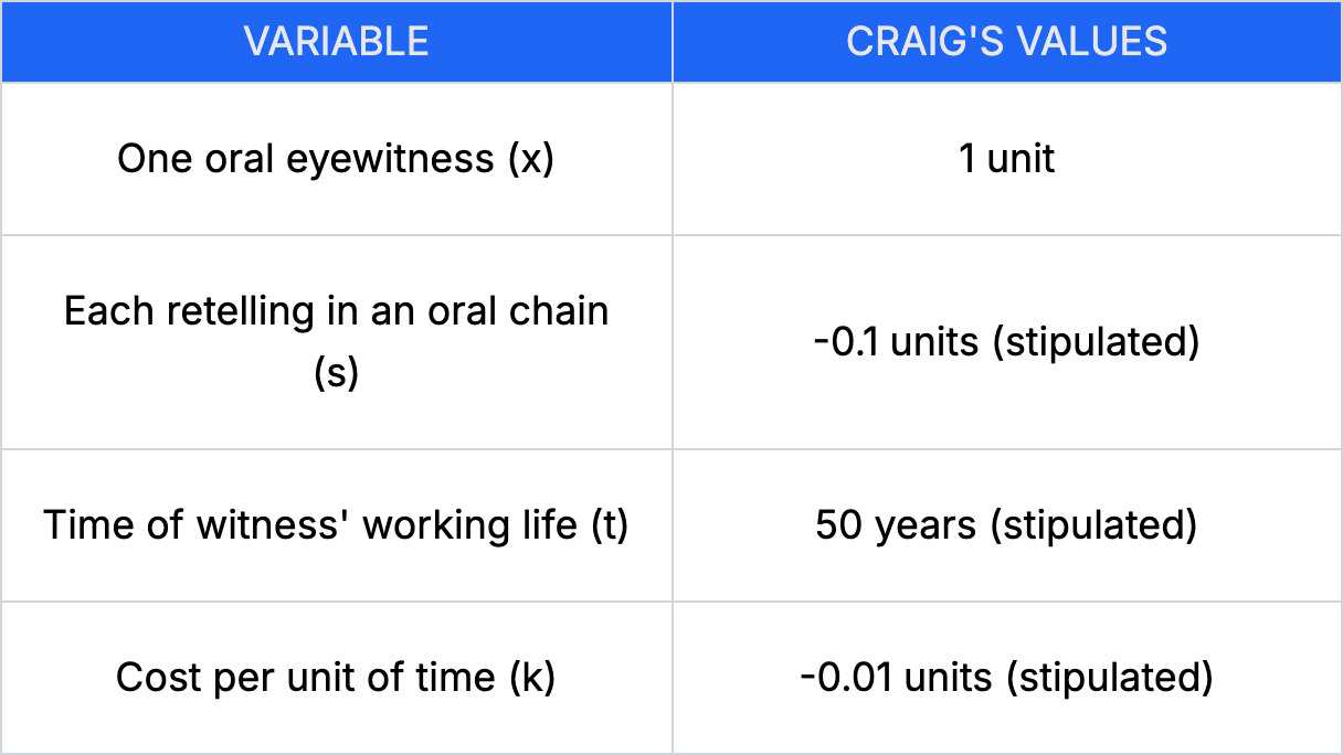
I left off the distance-related variables, because he thinks distance is only relevant for permanent things that one could go check on, not transient things (for example an event, like a battle). As we will see, distance won’t be relevant for his really important claim. It is absent from all the following equations, and the focus is on the time effect.
First, let’s put Craig’s equation to the test, using an example he provides. Imagine that instead of the Apostles writing Gospels, they only transmitted it orally. We want to figure out when the evidence would have lost its value, so set P = 0.
Matthew, Mark, Luke, and John…okay, so b = 4. Also, x is just our unit, and we can set it to 1, so 4 x 1 = 4. Remember that s = -0.1. We can simplify the time effect:
So, we are left with:
Now for some good old algebra. Multiply every term by 100 (Craig wanted integers — remember, no calculators in 1699.) That gives us 400 − 10(u − 1) − u² = 0. Distribute the −10: 400 − 10u + 10 − u² = 0. Add that 10, 410 − 10u − u² = 0. Multiply through by −1 so the u² term is positive, which allows us to use the quadratic formula. u² + 10u − 410 = 0.
So, we have u = 15.86 which Craig rounds to 16.5 Remember, this u is not years, but blocks of 50 years after the event. So we get 16 x 50 = 800. This count should tell us when the oral accounts of Matthew, Mark, Luke, and John would lose their historical evidentiary value. By this math, that year is 800 A.D.
Now, Craig starts the count at ~ 0 A.D., when he should (it seems to me) be starting at 33 A.D. I think he does this because 800 A.D. is a really convenient date: it is the year when Charlemagne was crowned Emperor of the Romans on Christmas Day by Pope Leo III in Rome.6
The Eschatology of P
n.b. Stigler explains the math of Craig’s work much better than I do. Check his book out if you get a chance.
Craig had a specific application in mind for his equation: the Gospels. John Craig wanted to define when the probabilitas of the written tradition would reach 0, because of his reading of this Bible verse:
“Nevertheless when the Son of man cometh, shall he find faith on the earth?”7
Luke 18:8
Craig interpreted this to mean that when P reached zero, that would be (roughly) the time of the Second Coming. Craig, as a vicar in the Church of England, was also interested in countering radical Protestant claims about the imminent end of the world. To do this, Craig is also going to show us how many witnesses’ worth of evidence we had for the Gospels in 1696.
Unfortunately, this also means I need to introduce some new variables.
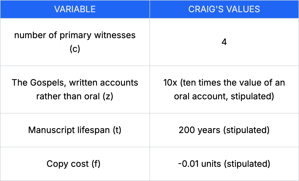
Some changes have to be made, because Craig wanted to account for differences between written and oral testimony. Each written Gospel is worth 10 times an oral account, which is an arbitrary judgment he made. He also guesses at manuscripts lasting about 200 years, and losing about 0.01 units per copy. Let’s see how Craig solves for P in 1696.
28x, which means that reading the Gospel in 1696 is equivalent to hearing about it from 28 eyewitnesses. This is less than the 40 eyewitnesses it was worth immediately after the life of Christ, but it’s hardly time to start saying a kyrie eleison.8 It is also a useful counter to the emerging Deist rejection of the resurrection: Craig is in this sense an apologist, demonstrating that there is still strong evidence for the Resurrection.
Finally, let’s find out when the Second Coming really will happen. I’m not going to walk through the math this time, because it mirrors what we did in the previous section.
The Second Coming is likely to occur around 3150 A.D., according to Craig. His argument is actually that Christ must come before this time, but will probably come around that moment because of his interpretation of Luke 18:8. He believes “when the Son of man cometh, shall he find faith on the earth?” implies that:
“so little…will be the probability [probabilitatis] of his story at the coming of Christ that he doubts whether he will find anyone who will give faith to this history concerning himself. Whence it is apparent how gravely in error are all those who fix the coming of Christ so near to our times.”
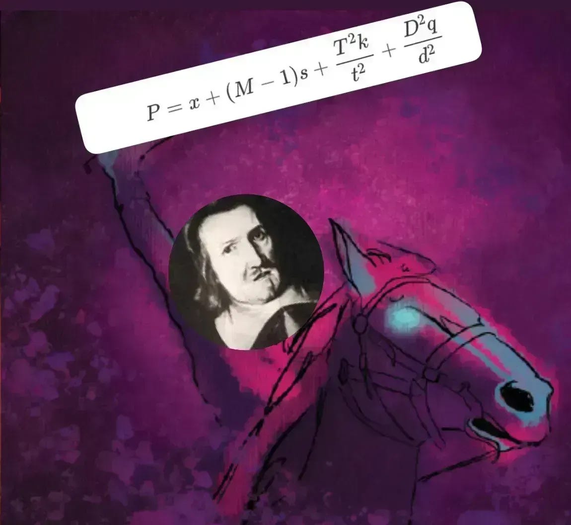
Now let’s briefly turn to the mathematical ramifications of Craig’s futurecasting.
Precociously Logarithmic?
It would be a mistake to try to read the future of mathematics and probability into Craig’s work (like I do in the title of this section). It’s not useful to think of practitioners of math or science working within an earlier paradigm as getting “close” to a “correct” answer, or “anticipating” the future. Much more compelling is how Craig identified and attempted to solve the same problems that motivated logistic regression.
Stephen Stigler in particular is convinced that John Craig pursues a solution isomorphic to the Log-Likelihood Ratio with his P variable. Craig is attempting to describe changes in the weight of evidence produced by data, and he attempts to use an additive measure with a baseline of 0. So Craig’s P isn’t a bad attempt to measure probability, it is an attempt to create something like a Log-Likelihood Ratio before there was a formalized method. When interpreted this way, Stigler notices that his equation also starts to look a lot like logistic regression: posterior log odds = starting value + (something × witnesses) + (something × time²) + (something × distance²).
All that said, this resemblance is mostly superficial. It is true that Craig stumbled on to something that looks a lot like logistic regression, but he didn’t understand it. First of all, Craig didn’t think that his P should go negative because you cannot have negative witnesses, so he asserts that it approaches zero without ever becoming negative. Conversely, the whole point of log odds is that they do become negative (between -∞ and ∞). Secondly, logistic regressions are binary, and Craig’s historical probability isn’t yes/no, but a measure of assent.9
Predicting the Future with Numbers
We should not be surprised that early modern attempts to predict the future using math were fraught. Probability had only just emerged as a field and calculus was new when Craig was writing. And yes, Craig’s calculations obviously don’t make a lot of sense to us now. By incorporating Newtonian physics into his calculations, Craig is applying geometry to moral objects; his T² suggests that doubt is continually accelerated by time because he wants it to behave like gravity.10 Now we don’t construct models like this, but Craig was operating under an entirely different paradigm.
Craig is a compelling figure. He was bold enough to attempt to implement the idea that we can quantify our belief (or credence) in some claim. This idea existed in Leibniz and Locke, but no maniac was willing to come up with some coefficients, be honest about them, and do the math until Craig. In the eighteenth century it would be improved upon significantly by Thomas Bayes, but mathematicians like Craig laid the groundwork. And since we’ve become accustomed to more opaque models which are reliant on conventional values we can appreciate that Craig had the decency to admit his arbitrary values were arbitrary. Good luck finding that on Substack.
Bibliography
Craig, Joannis. “Theologiae Christianae Principia Mathematica.” Translated in History and Theory 4 (1964): 1–31. https://doi.org/10.2307/2504310.
Stigler, Stephen. Statistics on the Table: The History of Statistical Concepts and Methods. Cambridge, MA: Harvard University Press. 1999, 252-273.
This isn’t actually a recent phenomenon at all. People have been fascinated with the probability of miracles since the eighteenth century.
See Stigler, 254.
The model that Locke lays out is more complicated than the model that Craig creates. Locke’s model includes incorporating any evidence of contradictory stories, the intelligence of witnesses, and certain other things that would have proven much more difficult to model.
“sint quantitates cognitae; sunt enim totidem unitates ad mensurandam Probabilitatem necessariae; quae proinde (sicut in omni alio mensurationis genere) ad arbitrium mensurantis assumi possunt.” This is how Craig describes creating his units. It is an interesting problem: he intentionally conflates the arbitrary nature inherent to creating units (like meters) with a coefficient which is supposed to describe the world.
The math savvy among you might notice that we also have u₂. Negative u is negative time, so it doesn’t make sense in Craig’s formulation. Basically, it just didn’t occur to him to specify his domain u ≥ 0.
It might be that Craig (a vicar in the CoE) was intentionally critiquing Catholic claims to carry on a tradition outside of scripture.
Evidently he chose to ignore the question mark.
This gives us about 23 eyewitnesses in 2026. Tick-tock.
I don’t want to just catalogue the problems with Craig’s work, but of course there are a bunch. One important one is that Craig simply charges a 0.1 cost for each retelling, when he would be creating a more accurate model with a Markov Chain. If he could have possibly known what that was.
I don’t get into this in this article, but this is where distance becomes important for Craig’s argument. The incorporation of distance allows him to imitate the structure of Newtonian physics.
Interesting article ! I wonder if there's been any more modern attempts at this argument. And I was impressed you used LaTeX lol (altho one eqn showed up as a "missing \end{aligned}")
Great article! I was wrong.